#StandWithUkraine - Stop the Russian invasion
Join us and donate. Since 2022 we have contributed over $5,000 in book royalties to Save Life in Ukraine & Ukraine Humanitarian Appeal & The HALO Trust, and we will continue to give!
Match Columns with XLOOKUP
Spreadsheet tools also allow you to “look up” data in one sheet and automatically find and paste matching data from another sheet. This section introduces the XLOOKUP function, where the “X” stands for “cross,” meaning matches across columns, which is the most common way to look up data. You’ll learn how to write a function in one sheet that looks for matching cells in select columns in a second sheet, and pastes the relevant data into a new column in the first sheet. If you’ve ever faced the tedious task of manually looking up and matching data between two different spreadsheets, this automated method will save you lots of time.
Tip: Earlier editions of this book described a similar function called VLOOKUP, but the XLOOKUP function is simpler to set up and more flexible. See more about both in the Google Sheets help page for XLOOKUP and the help page for VLOOKUP.
Here’s a scenario that illustrates why and how to use the XLOOKUP function. Figure 2.35 shows two different sheets with sample data about food banks that help feed hungry people in different parts of the US, drawn from Feeding America: Find Your Local Food Bank. The first sheet lists individual people at each food bank, the second sheet lists the address for each food bank, and the two share a common column named organization. Your goal is to produce one sheet that serves as a mailing list, where each row contains one individual’s name, organization, and full mailing address. Since we’re using a small data sample to simplify this tutorial, it may be tempting to manually copy and paste in the data. But imagine an actual case that includes over 200 US food banks and many more individuals, where using an automated method to match and paste data is essential.
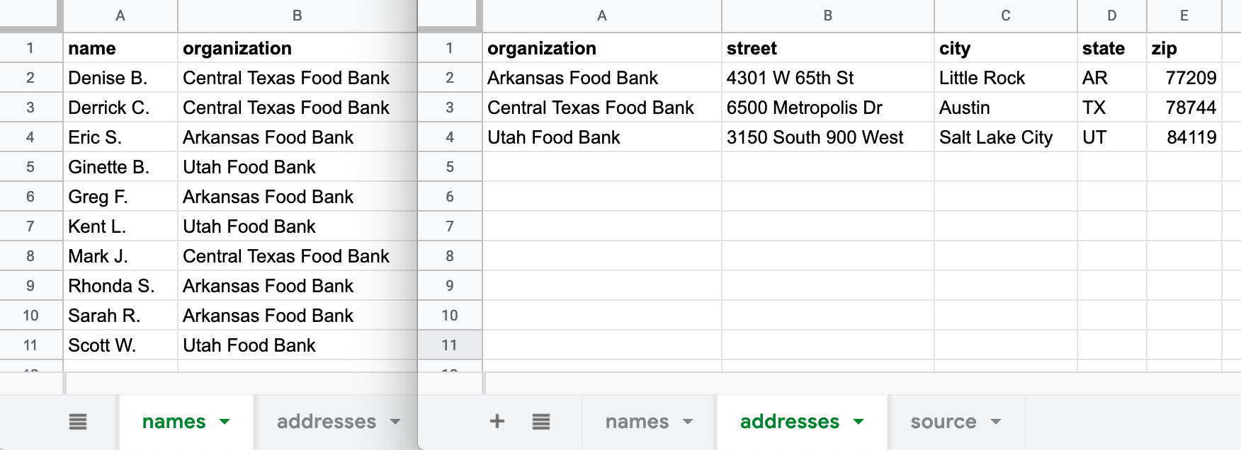
Figure 2.35: Your goal is to create one mailing list that matches individual names and organizations on the left sheet with their addresses on the right sheet.
- Open this Google Sheet of Food Bank sample names and addresses in a new browser tab. Log into your Google Drive, and go to File > Make a Copy to create your own version that you can edit.
We simplified this two-sheet problem by placing both tables in the same Google Sheet. Click on the first tab, called names, and the second tab, called addresses. In the future, if you need to move two separate Google Sheets into the same file, go to the tab of one sheet, right-click the tab to Copy to > Existing spreadsheet, and select the name of the other sheet.
- In your editable copy of the Google Sheet, the names tab will be our destination for the mailing list we will create. Go to the addresses sheet, copy the column headers for street - city - state - zip, and paste them into cells C1 through F1 on the names sheet, as shown in Figure 2.36. This creates new column headers where our lookup results will be automatically pasted.
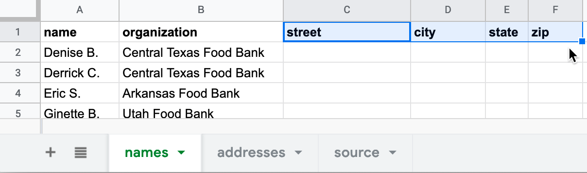
Figure 2.36: Paste the last four column headers from the addresses sheet into the names sheet.
- In the names sheet, click in cell C2 and type
=XLOOKUP, and Google Sheets will suggest that you complete the full formula in this format:
XLOOKUP(search_key, lookup_range, result_range,...)Here’s what the three required parts mean:
- search_key = The cell in 1st sheet you wish to match.
- lookup_range = The column or row in the 2nd sheet to search for your match.
- result_range = The column or row the 2nd sheet that contains your desired result.
Afterwards are three optional parts, which in most cases you can omit and use the default values: - missing_value = The value to return if no match is found (#N/A by default). - match_mode = The precision level for finding matches (default is 0 for exact match). - search_mode = The direction for searching matches (default is 1 from first to last).
- One option is to directly type this formula into cell C2, using comma separators, but it’s very long:
=XLOOKUP(B2,'addresses'!A:A, 'addresses'!B:B).
A better option is to click on the XLOOKUP cross lookup green box that Google Sheets suggests, and click on the relevant cells, columns, and sheets for the formula to be automatically entered for you, as shown in Figure 2.37. What’s new here is that this formula in the names sheet refers to a range of all rows in columns A and B in the addresses sheet. Press Return or Enter on your keyboard.
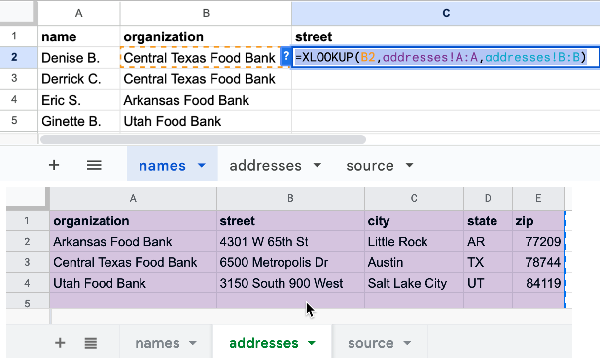
Figure 2.37: The XLOOKUP formula in cell C2 of the names sheet (top) searches for matches across column A in the addresses sheet and shows results from column B (bottom).
Let’s break down each part of the formula you entered in cell C2 of the names sheet:
B2= The search_key: the cell in the organization column of the names sheet you wish to match.'addresses'!A:A= The lookup range where you are searching for a match in the organization column of the addresses sheet.'addresses'!B:B= The result range, meaning your desired result in the street column of the addresses sheet.
- After you enter the full XLOOKUP formula, it will display the exact match for the first organization, the Central Texas Food Bank, whose address is 6500 Metropolis Dr. Click and hold down on the blue dot in the bottom-right corner of cell C2, and drag your crosshair cursor across columns D to F and let go, which will automatically paste and update the formula for the city, state, and zip columns, as shown in Figure 2.38.
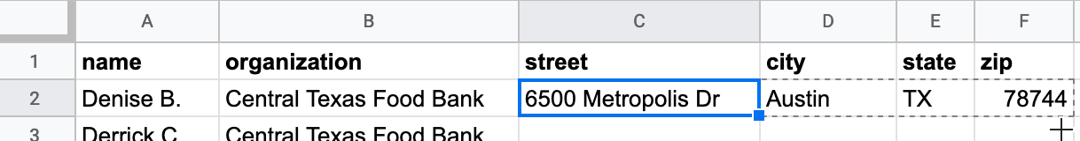
Figure 2.38: Click on cell C2, then hold-and-drag the bottom-right blue dot across columns D to F, which automatically pastes and updates the formula.
- Finally, use the same hold-and-drag method to paste and update the formula downward to fill in all rows, as shown in Figure 2.39.
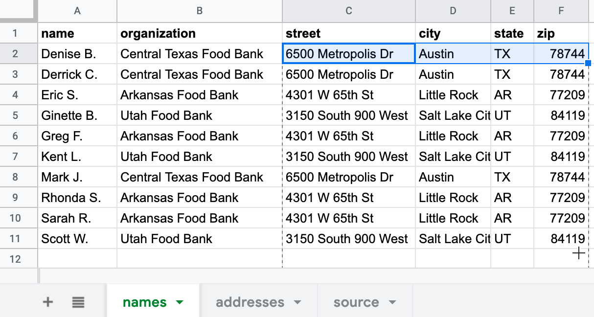
Figure 2.39: Click on cell F2, then hold-and-drag the bottom-right blue dot down to row 11, which automatically pastes and updates the formula.
Warning: If you save this spreadsheet in CSV format, your calculated results will appear in the CSV sheet, but any formulas you created to produce those results will disappear. Always keep track of your original spreadsheet to remind yourself how you constructed formulas.
You’ve successfully created a mailing list—including each person’s name, organization, and full mailing address—using the XLOOKUP function to match and paste data from two sheets. Now that you understand how to use formulas to connect different spreadsheets, the next section will teach you how to manage multiple relationships between spreadsheets with the help of a relational database.