Calculate with Formulas

#StandWithUkraine - Stop the Russian invasion

Join us and donate. We are contributing all book royalties from 2022 to present to:
Save Life in Ukraine and Ukraine Humanitarian Appeal.

Spreadsheet tools can save you lots of time when you insert simple formulas and functions to automatically perform calculations across entire rows and columns of data. In this section you’ll learn how to write formulas and functions in a sample dataset.

Always start a formula with an equal sign (=) to tell the spreadsheet tool you are inserting a calculation, rather than regular text or numbers. Simple formulas use symbols for mathematical operations between specific cells:

Plus symbol (+) to add, like this: = B2 + B3
Minus symbol (-) to subtract, like this: = B2 - B3
Asterisk symbol (*) to multiply, like this: = B2 * B3
Forward slash (/) to divide, like this: = B2 / B3

Also, spreadsheet tools contain built-in functions that save us time by avoiding the need to write long formulas. Two simple functions are =SUM() and =AVERAGE(), which run calculations on cells inside the parentheses. A colon symbol (:) represents a consecutive range of cells. For example, the cells B2, B3, B4, B5, and B6 can be represented this like: (B2:B6).

To add up five cells, you could enter: = B2 + B3 + B4 + B5 + B6
But this function is faster: =SUM(B2:B6)
To find the average of five cells, you could enter: = ( B2 + B3 + B4 + B5 + B6 ) / 5, using parentheses to add up the sum before dividing by the count of numbers
But this function is faster: =AVERAGE(B2:B6)

Tip: Instead of typing out each character in your formulas and functions, experiment by clicking on specific cells or column headers, or clicking and dragging across ranges of cells, to automatically enter your desired instructions. For example, when you start typing the function =AVERAGE(), instead of typing B2:B6 inside the parentheses, you can click on cell B2, hold down your mouse or trackpad button, and drag to B6. Your spreadsheet tool should automatically generate this formula: =AVERAGE(B2:B6).

Now let’s practice our formula skills using the reader survey sample dataset described at the top of the chapter. You’ll use one function to calculate an average numeric value, and another function to count the frequency of a specific text response.

Open this Google Sheet of Hands-On Data Visualization reader public survey responses in a new tab in your browser.
Log into your Google Drive account, and go to File > Make a Copy to edit your own version.
Add a blank row immediately below the header to make space for our calculations. Right-click on row number 1 and select Insert 1 below to add a new row, as shown in Figure 2.26.

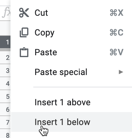
Figure 2.26: Right-click on row number 1 and select Insert 1 below.

Let’s calculate the average level of reader experience with data visualization. Click on cell E2 in the new blank row you just created, and type an equal symbol (=) to start a formula. Google Sheets will automatically suggest possible formulas based on the context, and you can select one that displays the average for current values in the column, such as =AVERAGE(E3:E2894), then press Return or Enter on your keyboard, as shown in Figure 2.27.

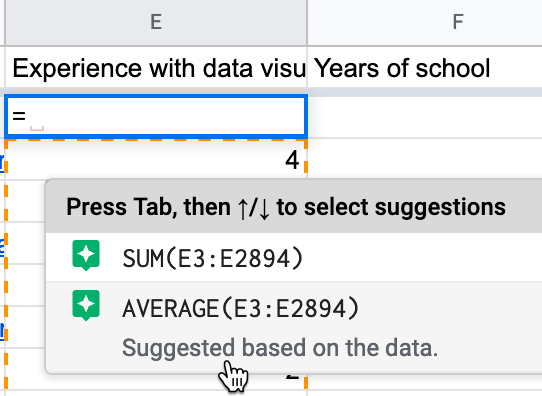
Figure 2.27: Type = to start a formula and select the suggestion for average, or type it directly in with the correct range.

Since our live spreadsheet has a growing number of survey responses, you will have a larger number in the last cell reference to include all of the entries in your version. Currently, the average level of reader experience with data visualization is around 2 on a scale from 1 (beginner) to 5 (professional), but this may change as more readers fill out the survey. Note that if any readers leave this question blank, spreadsheet tools ignore empty cells when performing calculations.

Tip: In Google Sheets, another way to write the formula above is =AVERAGE(E3:E), which averages all values in column E, beginning with cell E3, without specifying the last cell reference. Using this syntax will keep your calculations up-to-date if more rows are added, but it does not work with LibreOffice or Excel.

Part of the magic of spreadsheets is that you can use the built-in hold-and-drag feature to copy and paste a formula across other columns or rows, and it will automatically update its cell references. Click in cell E2, and then press and hold down on the blue dot in the bottom-right corner of that cell, which transforms your cursor into a crosshair symbol. Drag your cursor to cell F2 and let go, and show in Figure 2.28. The formula will be automatically pasted and updated for the new column to =AVERAGE(F3:F2894) or AVERAGE(F3:F), depending on which way you entered it above. Once again, since this is a live spreadsheet with a growing number of responses, your sheet will have a larger number in the last cell reference.

Figure 2.28: Click on the blue bottom-right dot in cell E2, then hold-and-drag your crosshair cursor in cell F2, and let go to automatically paste and update the formula.

Since the Occupation column contains a defined set of text responses, let’s use a different function to count them using an if statement, such as the number of responses if a reader listed “educator”. Click in cell G2 and type the equal symbol (=) to start a new formula. Google Sheets will automatically suggest possible formulas based on the context, and you can select one that displays the count if the response is educator for current values in the entire column. You can directly type in the formula =COUNTIF(G3:G2894,"=educator"), where your last cell reference will be a larger number to reflect all of the rows in your version, or type in the Google Sheets syntax =COUNTIF(G3:G,"=educator") that runs the calculation on the entire column without naming a specific endpoint, as shown in Figure 2.29.

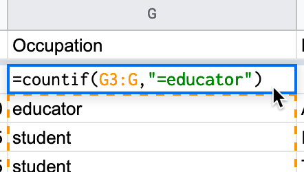
Figure 2.29: Select or enter a formula that counts responses if the entry is educator.

Spreadsheet tools contain many more functions to perform numerical calculations and also to modify text. Read more about functions in this support pages for Google Sheets, LibreOffice, or Microsoft Excel support page.

See additional spreadsheet skills in later chapters of the book, such as how to find and replace with blank, split data into separate columns, and combine data into one column in Chapter 4: Clean Up Messy Data. See also how to normalize data in Chapter 5 and how to pivot address points into polygons in Chapter 13: Transform Your Map Data.

Now that you’ve learned how to count one type of survey response, the next section will teach you how to regroup data with pivot tables that summarize all responses by different categories.